Hysteresis loop of a magnetic nanoparticle in an AC field
This page solves Brown’s Fokker–Planck equation for the orientation distribution W(θ, t) of a single-domain, uniaxial nanoparticle whose easy axis is aligned with the alternating field and whose body is immobilised (Néel relaxation only, no Brownian rotation). The periodic steady state gives the dynamic loop m(H), the specific absorption rate and the efficiency ε = SAR/SARmax relative to the fundamental bound SARmax = 4 μ0MsC/ρ at the field–frequency limit H0 f = C. Reference: D. Suess et al., Reaching fundamental limits of magnetic nanoparticles for hyperthermia (2026, in preparation).
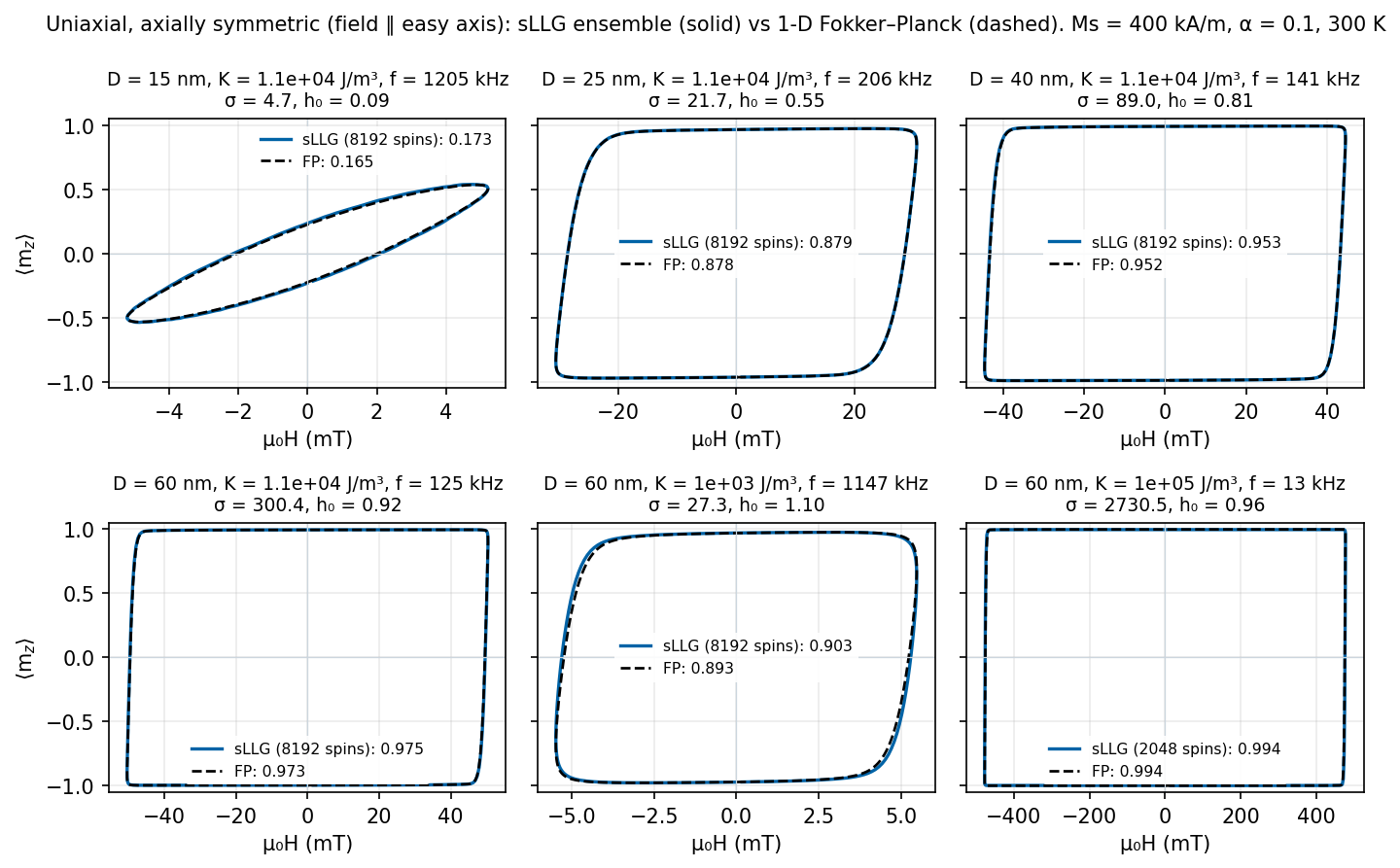
Everything on this page is computed live in your browser from the equation below (Web Worker, no server, no lookup tables); the Python reference solver gives identical numbers (ε = 0.878 for the default case).
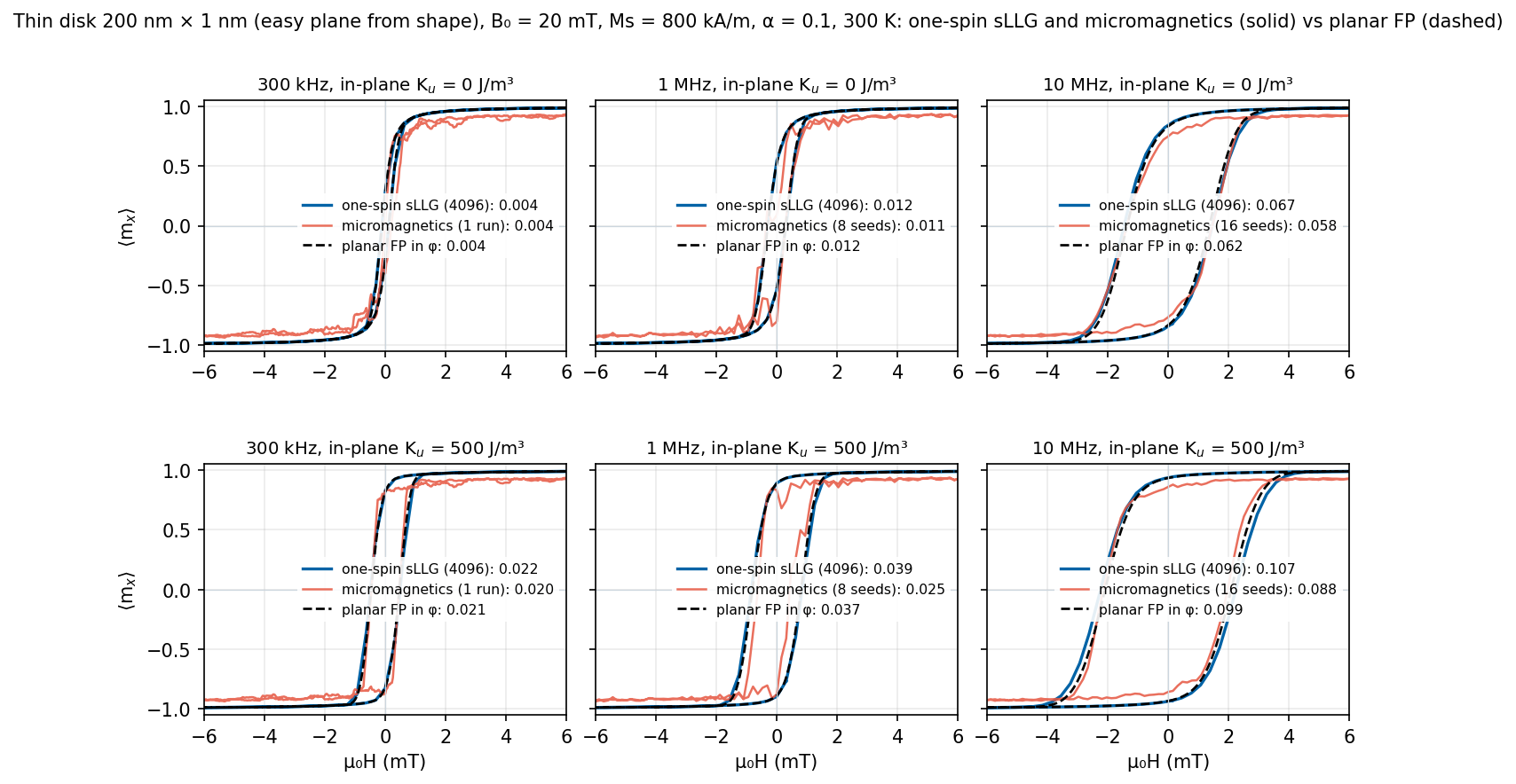
Companion applet: thin disk as one spin with a strong easy plane (MPI and hyperthermia) →
How the model works: what is computed, the energy, the unknown W(x,t), the equation, symbols, numericsfor a physicist who has not read the paper
What is computed
A single-domain nanoparticle with uniaxial anisotropy sits in an alternating field H(t) = H0 sin(2πf t) applied along its easy axis. The particle is immobilised (no mechanical or Brownian rotation of the particle body) and does not interact with neighbours, so the only degree of freedom is the direction of its magnetic moment μ = MsV, which fluctuates thermally between the two easy directions and is driven back and forth by the field. The applet solves Brown’s Fokker–Planck equation for the probability density of that direction, live in your browser (nothing is precomputed, nothing runs on a server), and integrates the dynamic hysteresis loop of the ensemble average m(t) = ⟨cos θ⟩ over one field period. The area of the loop is the energy dissipated per cycle; from it follow the specific absorption rate SAR and the efficiency ε relative to the bound SARmax.
The energy landscape
With θ the angle between the moment and the easy axis (which is also the field axis), the energy is the sum of anisotropy and Zeeman terms,
E(θ) = K1 V sin²θ − μ0 Ms V H(t) cos θIn units of kBT, with x = cos θ, the reduced field h = H/HK, HK = 2K1/(μ0Ms) and the reduced barrier σ = K1V/kBT:
E/kBT = σ sin²θ − 2σ h cos θ = σ(1 − x²) − 2σ h xFor |h| < 1 there are two minima, θ = 0 (x = +1, energy −2σh) and θ = π (x = −1, energy +2σh), separated by a maximum at x = −h. Seen from the well aligned with the field the barrier is σ(1 + h)², seen from the well opposed to the field it is σ(1 − h)²: the field lowers one barrier and raises the other, which is what drives the moment across. At h ≥ 1 the opposed minimum disappears altogether and the moment switches deterministically — the Stoner–Wohlfarth limit, which the loop approaches for large σ (large particles, low temperature, high frequency).
The unknown: W(x, t)
W(x, t) is a probability density in one orientation variable, x = cos θ ∈ [−1, 1], and time: W(x,t) dx is the probability that the projection cos θ of the moment onto the axis lies in [x, x+dx] at time t. Because the field is parallel to the easy axis the problem is axially symmetric: the azimuth φ of the moment carries no information and has been integrated out, so W is a function of just two variables and is normalised, ∫−1+1 W dx = 1. W is not the magnetisation; the magnetisation is its first moment m(t) = ∫ x W(x,t) dx = ⟨cos θ⟩ = M(t)/Ms. The heat map in the panel “Distribution W(x, t)” shows W itself; the loop is m plotted against h.
The equation
∂W/∂t = (1 / 2τN) ∂/∂x [ (1 − x²) ( ∂W/∂x + W ∂(E/kBT)/∂x ) ]This is a drift–diffusion (Smoluchowski) equation on the unit sphere. The first term in the inner bracket is diffusion: thermal agitation spreading the orientation. The second is drift: the torque −∂E/∂θ pulling the moment towards the energy minima. The factor (1 − x²) = sin²θ is the metric of the sphere in the variable x; it makes the flux vanish at the poles, so probability is conserved. The single time constant is the free rotational diffusion time of the moment,
τN = (1 + α²) Ms V / (2 α γ kBT) = σ τ0, τ0 = (1 + α²) / (α γ Bani), Bani = 2K1/Ms, γ = 1.760859×10¹¹ rad s−1 T−1Brown (1963) derived this equation as the exact orientation-space form of the stochastic Landau–Lifshitz–Gilbert equation for this geometry — it is the same physics as a thermal LLG simulation of one macrospin, but for the full ensemble at once and without noise. The smallest non-zero eigenvalue of the operator at fixed field is the Néel relaxation rate 1/τ; the familiar two-level (Arrhenius) master equation, τ ∝ τ0 exp[σ(1 ∓ h)²], is its high-barrier limit. Here no such approximation is made: the full distribution is propagated for any σ, h and frequency, including the superparamagnetic and the Stoner–Wohlfarth regimes and everything in between.
Symbols
| Symbol | Meaning | Unit · how it enters |
|---|---|---|
| K1 | uniaxial anisotropy constant | J/m³ · barrier K1V and anisotropy field HK |
| V = πD³/6, D | magnetic core volume and diameter | m³, nm · σ ∝ V, τN ∝ V |
| Ms | saturation magnetisation | A/m · Zeeman energy, HK, SAR prefactor |
| α | Gilbert damping | – · time scale τ0 only |
| γ | gyromagnetic ratio, 1.760859×10¹¹ | rad s−1T−1 · τ0 |
| T, kBT | temperature, thermal energy | K, J · σ and τN |
| ρ | mass density of the particle | kg/m³ · converts power per volume to SAR per mass |
| H(t) = H0 sin 2πft | applied field along the easy axis | A/m (μ0H in mT) · drive |
| H0, f | field amplitude and frequency | A/m, Hz · inputs; H0f compared with C |
| HK = 2K1/(μ0Ms) | anisotropy (Stoner–Wohlfarth switching) field | A/m · field unit of the reduced problem |
| h = H/HK, h0 = H0/HK | reduced field and amplitude | – · enters E/kBT as −2σhx |
| σ = K1V/kBT | reduced anisotropy barrier | – · controls blocking; τN = στ0 |
| τ0 = (1+α²)/(αγBani) | attempt-time scale, Bani = 2K1/Ms | s · prefactor of τN |
| τN = στ0 | free rotational diffusion time of the moment | s · the only time constant of the equation |
| E(θ) | energy of the moment (anisotropy + Zeeman) | J · drift term through ∂(E/kBT)/∂x |
| θ, x = cos θ | angle to the easy/field axis and its cosine | rad, – · the single orientation variable |
| W(x, t) | orientation probability density | – · the solved quantity, ∫W dx = 1 |
| m(t) = ∫ x W dx | reduced magnetisation M/Ms along the axis | – · first moment of W; plotted against h |
| A = −∮ m dh | loop area | units of MsHK · energy per cycle and volume = μ0MsHKA |
| SAR = f A μ0MsHK/ρ | specific absorption rate | W/kg (shown in W/g) |
| C = H0·f | field–frequency (patient discomfort) limit | A m−1s−1 · default 5×10⁹ |
| SARmax = 4μ0MsC/ρ | upper bound: square loop of full height at H0f = C | W/kg |
| ε = SAR/SARmax | efficiency; equals A/(4h0) when H0f = C | – · 0 … 1 |
| Hc | coercive field: |H| where m = 0 on the descending branch | A/m (μ0Hc in mT) |
| Mr | remanence: m at H = 0 | units of Ms |
Beyond the axially symmetric case (sphere modes)
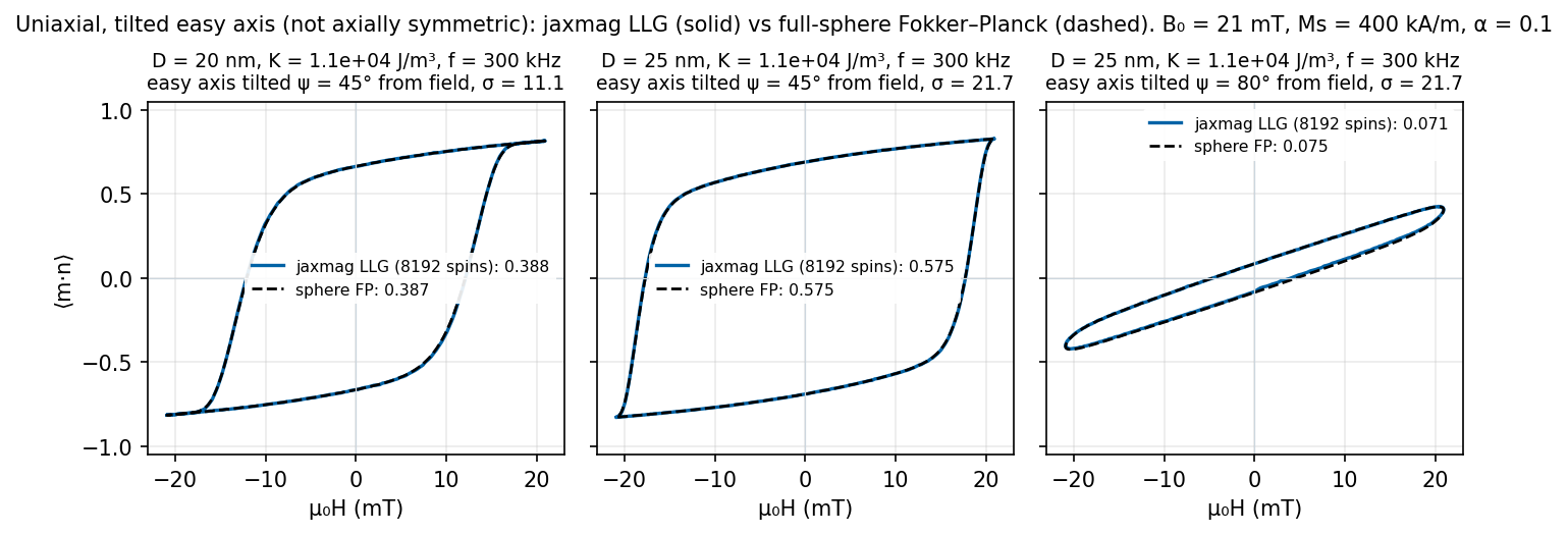
If the easy axis is tilted by ψ from the field, or the anisotropy is cubic, the azimuth no longer drops out and W depends on both angles. The mode selector then switches to Brown’s equation on the full unit sphere,
∂W/∂t = −∇s·(v W) + D ∇s²W, v = −γ' m×B − αγ' m×(m×B), D = αγkBT/((1+α²)MsV) = 1/(2τN), B = −(1/Ms)∂F/∂m + μ0H(t) nThe first term of v is the precession about the effective field. In the axially symmetric case it only rotates W about the axis and drops out; with tilted or cubic minima it couples the two angles and is essential (it is the reason why a tilted particle is not simply a projected 1-D one). Numerically, damping drift and diffusion use Scharfetter–Gummel fluxes, the precession uses central fluxes (upwinding it would add a large artificial diffusion when the minima lie away from the grid poles). Central fluxes are not monotone: when an energy well becomes narrower than about two cells (q = Δθ√σ > 0.6) W can turn negative, and the status line flags such results.
Cubic anisotropy: F = K1(mx²my² + my²mz² + mz²mx²) + K2mx²my²mz². For K1 < 0 (magnetite, K1 ≈ −1.1×10⁴ J/m³) the eight ⟨111⟩ directions are minima and the barrier between neighbouring minima (over ⟨110⟩) is only |K1|V/12, compared with KV for a uniaxial particle — a cubic magnetite particle of the same volume is therefore much more superparamagnetic. The field direction in the crystal frame can be chosen ([111], [100], [110]) or averaged over six quasi-uniform (Fibonacci) directions. Ms = 400 kA/m is the paper’s value; bulk magnetite has about 480 kA/m. For tilted uniaxial particles see I. S. Poperechny, Yu. L. Raikher, V. I. Stepanov, Phys. Rev. B 82, 174423 (2010).
Numerics in the browser: finite volumes on an Nθ×2Nθ grid (default 32×64), implicit Euler with 400 steps per period; each step is solved exactly with a band LU (bandwidth 2Nθ; the unresolved precession, ~10 rad per step, defeats Krylov solvers), the factors of the S/2+1 distinct step matrices are kept in float32 (~110 MB at 32×64) and every solve is finished by float64 iterative refinement; the periodic state comes from GMRES on (I − R Mhalf)W = 0 with R the inversion m → −m (typically two iterations). A loop takes 3–6 s (×6 for the orientation average).
Numerics — what “live” means
The interval x ∈ [−1, 1] is divided into N finite-volume cells uniform in θ (fine near the poles, where the population sits at large σ). Fluxes between cells use the Scharfetter–Gummel (exponentially fitted) scheme, so the discrete equilibrium is exactly the Boltzmann distribution for any σ. Time stepping is Crank–Nicolson with S steps per period, one tridiagonal solve per step. The periodic steady state is not reached by cycling until transients die out: the propagator over half a period, Mhalf, is assembled column by column, and the symmetry of the equation under (x, h) → (−x, −h) turns the periodicity condition into W* = R Mhalf W* with R the reflection x → −x. One dense N×N linear solve, with one row replaced by the normalisation, gives W*. From W* one period is propagated to record m(t), h(t) and W(x, t), whose normalisation is checked at every step (see the status line). With the defaults (N = 120, S = 600) this takes about 60 ms in a Web Worker, so every input change recomputes immediately. Crank–Nicolson is A-stable but not L-stable: when a large field (h0 > 1) sweeps the barrier of the opposed well from ≈25 kBT to zero within only a few time steps, the switching front is unresolved in time and the solution rings (negative W, |m| > 1). The applet therefore counts the steps in that sweep window, n = S √(25/σ) / (2π √(h0²−1)), and raises S automatically to the smallest multiple of 600 (at most 24 000) that gives n ≥ 20; the status line says so when it happens.
Steady-state loop m(H)
Distribution W(x, t)
vertical axisThe solved quantity: probability density of the moment orientation over one field period; the loop above is its first moment. Colour = log10 W; vertical axis x = cos θ (+1: along the field axis, −1: opposite) or θ (0° top, 180° bottom, uniform in the grid cells, better for large σ); thin line = h(t)/h0 (+1 top, −1 bottom).
Snapshots W(x)
Distribution W(φ, t)
The solved quantity (disk): probability density of the in-plane angle φ over one field period; the loop is its first harmonic ⟨cosφ⟩. Colour = log10 W; φ = 0 (along +x, the field axis) in the middle, ±180° at the edges; thin line = h(t)/h0.
Full sphere F(m), W(θ,φ,t)
Equirectangular maps of the unit sphere in the crystal frame (θ = 0° top, 180° bottom; φ = 0…360° left to right). Left: anisotropy energy F(m)/kBT (bright = low; circles = minima, + = field direction n, × = −n, ◇ = uniaxial axis). Right: log10 W (four decades below the maximum) at the selected time (for the orientation average: the first direction).
energy landscape
distribution W at t/T = 0.25
One period
m(t)/Msh(t)/h0Efficiency scan
H0 = C/f, 40 log-spaced pointsAppendix: validation against stochastic LLG — hysteresis loops for all model types
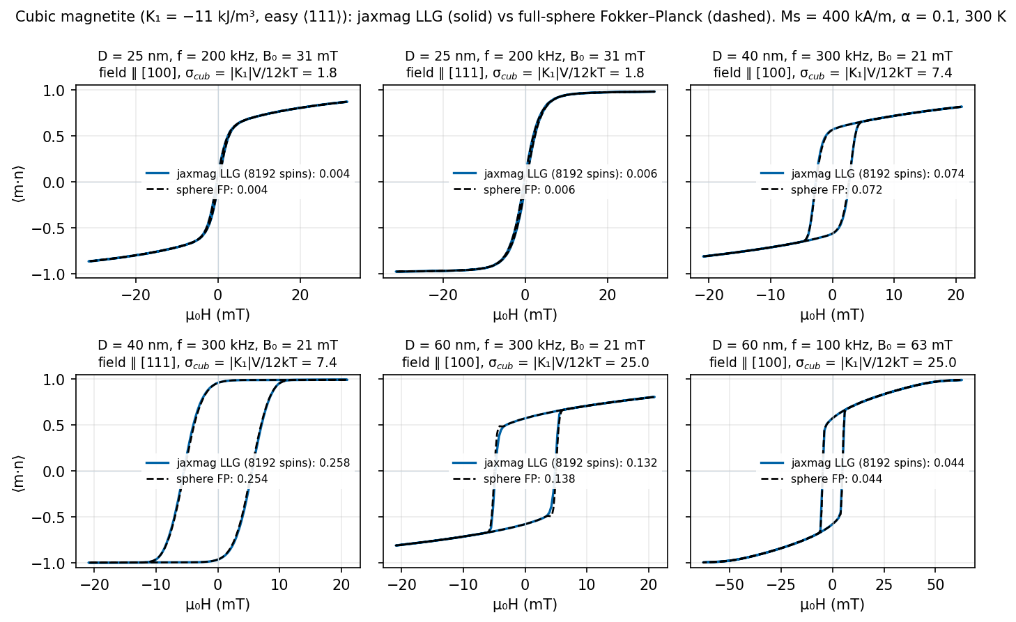
Hysteresis loops: stochastic LLG (solid) vs Fokker–Planck (dashed)
Each panel shows the steady-state loop of the ensemble-averaged magnetisation along the field; the legend gives the loop area / 4B0 computed from the plotted curve. Ms = 400 kA/m (particles) or 800 kA/m (disks), α = 0.1, T = 300 K throughout.
Cubic points in numbers
The full-sphere Fokker–Planck mode was checked against stochastic Landau–Lifshitz–Gilbert simulations with jaxmag (matrix-free cubic anisotropy operator make_cubic_anisotropy, ensembles of 8192 independent macrospins, Heun scheme, Δt = 1 ps, 4 field periods with the first discarded, run on the A100 GPUs of gto4). Material: cubic magnetite K1 = −1.1×10⁴ J/m³, K2 = 0, Ms = 4×10⁵ A/m, α = 0.1, T = 300 K, field on the discomfort limit H0f = C = 5×10⁹ A m−1s−1. Fokker–Planck on a 96 × 192 grid, 600 steps per period.
| point (area / 4B0) | Fokker–Planck | stochastic LLG (jaxmag) | difference |
|---|---|---|---|
| 25 nm, 200 kHz, 31.4 mT, field ∥ [111] | 0.0056 | 0.0056 ± 0.0001 | 0 % |
| 25 nm, 200 kHz, field ∥ [100] | 0.0039 | 0.0039 | 0 % |
| 40 nm, 300 kHz, 20.9 mT, field ∥ [100] (x) / [001] (z) | 0.0723 / 0.0739 | 0.0740 | 2 % / 0.1 % |
| 40 nm, 300 kHz, field ∥ [111] | 0.254 | 0.258 | 1.8 % |
| 60 nm, 300 kHz, field ∥ [100] | 0.138 | 0.132 | 4 % |
| 60 nm, 100 kHz, 62.8 mT, field ∥ [100] | 0.0445 | 0.0444 | 0.2 % |
(a) Symmetry test: a field along x and along z must give the same loop. The grid prefers z (its poles); the difference shrinks from 3.5 % on 64 × 128 to 2 % on 96 × 192.
(b) Resolution: on the coarse browser grids the 60 nm points are not resolved (narrow wells away from the grid poles; the applet flags them red). Use the default browser grid for D ≤ 40 nm in cubic mode and the finer grid option for larger particles.
(c) Physics: pure cubic magnetite loses far less than a uniaxial particle with K = |K1| (25 nm: 0.004–0.006 vs 0.88; 40 nm: 0.07–0.26 vs 0.95), because the barrier between neighbouring ⟨111⟩ minima is only |K1|V/12. This agrees with N. A. Usov, M. S. Nesmeyanov, E. M. Gubanova, N. B. Epshtein, Beilstein J. Nanotechnol. 10, 305 (2019), doi:10.3762/bjnano.10.29, who find appreciable SAR for cubic magnetite only at 45–55 nm; real particles that heat well have additional shape or surface anisotropy (combined anisotropy: N. A. Usov, J. M. Barandiarán, J. Appl. Phys. 112, 053915 (2012), doi:10.1063/1.4749799).
Code: jaxmag, gitlab.com/dietersuess/jaxmag, branch feature/md, examples/cubic_macrospin_loop.py.